Silicon Photonics Laboratory

Name of the course	Online	Lecture	Exercises[1]	Lab
Silicon Photonics Lab	✓	✓	✗ (✓)	✓

[1] optional

The Silicon Photonics Laboratory is a twelve-weeks course for master or bachelor programs, where level of complexity and workload of the course depend on the program. It is organized in two parts. Part One is an virtual classroom education on the Finite Difference Time Domain Method (FDTD), the Vector Wave Propagation Method (VWPM) and a very brief introduction to the Python language. Part Two is the practical lab training where students design and simulate selected silicon photonic standard components with the FDTD and/or the VWPM.

Each lab is focussed on a specific photonic building block as shown in the table below. The contents are incremental and build up on each other. After a brief introduction to the theory of the building blocks, participants model and simulate photonic components and prepare a report at the end of each exercise.

The course utilizes the software packages MEEP and VWPM. Both simulators are available for single and multiprocessor Linux systems and free of charge. Versions of OptiFDTD and VWPM are available for Windows systems but students are highly recommended to use the Linux because the course material is built on a Linux environment. All required software packages are available for download on students personal computers.

Conceptually, the course is set up as an online course and participants are not tied to a classroom at all. To successfully complete the course, it is an advantage have completed the course Optics and Photonics or at least have a basic knowledge in the relevant theory. Programming skills are absolutely required.

Having completed the course successfully, students will understand the functionality and design parameters of the basic silicon photonic components. They'll be able to create a model, set up a simulation environment, optimize the design and analyze the performance of the device.

Lecture	Content	PDF
1	Classification of problems and finite differencing	[PDF]
2	Classification of systems and introduction to Fourier optics	[PDF]
3	Finite differencing schemes for partial differential equations	[PDF]
4	The Finite Difference Time Domain Method	[PDF]
5	The Beam Propagation Method	[PDF]
6	The Wave Propagation Method	[PDF]
7	The Vector Wave Propagation Method	[PDF]

Lab	Content	Download
1	Plane Wave and Gaussian Sources	[.tar.gz]
2	Reflection at plane interface	[.tar.gz]
3	Waveguides	[.tar.gz]
4	Splitters & Tapers	[.tar.gz]
5	Grating Couplers	-
6	Fabry Perot and Ring Resonators	-
7	Circular Grating Outcoupler	-

1. Free Space Propagation

Free space propagation of Continous and Gaussian Sources with variations in the propagation vector, wavelength (frequency) and spectral width. Perform a spectral analysis of plane waves and Gaussian beams for vertical and oblique incidence. Align the results with the Fourier Theory and investigate the effect of Perfectly Matched Layer (PML) or Absorbing Boundary Conditions (ABC). Simulate with time stepping and cw-solver. Discuss symmetry settings.

2. Plane Interface

Derive the Fresnel Coefficients from a simulation of reflected and transmitted field amplitudes over a range of spatial frequencies. Use a Gaussian Pulse to obtain the impulse response of the interface. Derive reflected and transmitted field amplitudes over the angle of incidence. Compared results to a simulation with plane waves. Develop an anti-reflection coating from impulse response analysis.

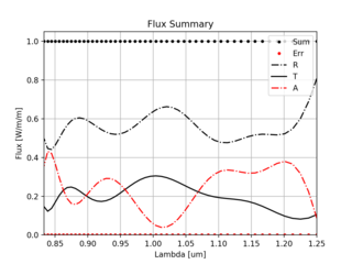
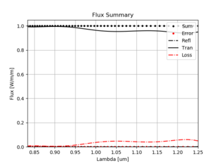
3. Waveguide

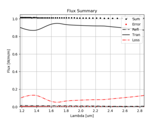
Model a Straight Waveguide and calculate radiation losses. Perform a variation of wavelength and contrast, i.e. refractive index ratio of core and cladding. Verify that mode confinement is only reached with total internal reflection and that only a discrete set of modes are carried by the waveguide due to phase alignment (resonance/standing wave) conditions at the waveguide boundaries. Optimize the waveguide for monomode propagation and analyze the energy flux. Plot transmittance and reflectance over spectral range.

Model and simulate a rectangular and circular Waveguide Bend and analyze the energy flux. Parametrize the bend and determine the maximum bend angle for mode confinement. Determine the normalized energy flux of transmitted fields over spatial frequency and determine the waveguide losses. Compare the performance of orthogonal and circular bend. Photonic Crystal Waveguides are optional if time permits.

4. Splitter & Taper

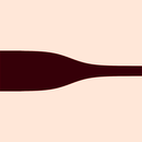
Model and optimize a Waveguide Splitter to achieve a maximum trans- mittance and compare performance for two design points. Optimize a Waveguide Taper to achieve a maximum transmittance. Understand how taper and splitter shapes (linear, exponential, etc.) affect their operability. Investigate how device performance is influenced by source misalignments. Perform parameter variations and performance evaluations.

5. Grating Coupler

Model and optimize a one-dimensional Grating Coupler. Analyze the spectrum of transmitted and reflected beam. Show the dependency of grating parameters to diffraction orders. Attach a waveguide to the grating and analyze the coupling efficiency. Explore the design space and identify an optimal solution for a maximum transmission. Investigate the interdependency of wavelength, angle of incidence and grating pitch (width).

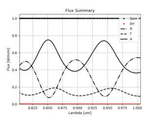
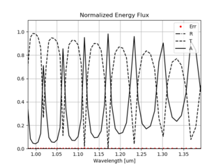
6. Fabry Perot & Ring Resonator

Investigate the theory of Fabry Perot resonators. Develop a Ring Resonator to selectively filter wavelengths. Use the theory of ring resonators to verify the conditions of resonance. Engineer a design to selectively filter one of two wavelengths. Use two Gaussian sources and perform a mode analysis of the input and output spectrum. Evaluate the results and optimize the design for a maximum mode separation. Use the material parameters and dimensions of a standard CMOS SOI technology.

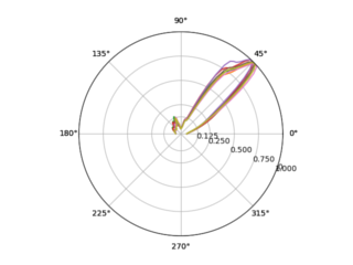
7. Nonlinear optimization of a bragg-grating outcoupler

This exercise is intended for participants with a solid background in Silicon Photonics, Optics and experience in Pyton and Shell programming. The bragg-grating outcoupler is designed in three dimensions. A parameter configuration shall be found for maximum outcoupling power using a nonlinear optimizer, e.g. nlopt. The corresponding radiation patterns are obtained from the Poynting vector in a far-field analysis. The optimizer is supposed find a power maximum for a user-defined range of angles.

Helpful Links

[1] MEEP install guide
[2] Python documentation for MEEP
[3] Python documentation for HDF5-Format
[4] Managing Python libraries with Anaconda
[5] MIT Photonic Bands (MPB)
[6] Python documentation for MIT Photonic Bands (MPB)
[7] NumPy Reference, a scientific computing package for Python
[8] About MEEP and VWPM.

Literature

[1] Principles Of Optics, Born & Wolf, Cambridge University Press, ISBN 0-521-64222-1
[2] Fourier Optics, Goodman, Roberts Publ., ISBN 0-974-70772-4
[3] The Finite-Difference Time-Domain Method, Taflove, Artech House Inc., ISBN 1-580-53832-0
[4] Engineering Optics With Matlab, Poon & Kim, World Scientific Publ. Co, ISBN 9-789-812-56873-1
[5] Optics, Hecht, Addison-Wesley Publ., ISBN 9-780-805-38566-3