The Vector Wave Propagation Method

Electromagnetic field distributions can be derived from closed analytic solutions only for simple problems. Real applications are complex so that closed analytic solutions do not exist. Hence, simulation methods are used to simulate electromagnetic field propagation. Such simulators approximate the partial differential equations that are obtained from the Maxwell equations. While finite difference time domain methods are very accurate but memory and time consuming and therefore primarily suitable for small systems, other methods like the split-step propagation scheme limit the propagating field to the paraxial regime. For instance the split-step BPM (Beam Propagation Method) is such a method. The split-step BPM is therefore applicable to paraxial spatial frequencies where the Fresnel coefficients and vector waves to not show significant differences to scalar waves.

The Wave Propagation Method (WPM) introduced by Brenner in 1993 overcomes the paraxial approximation. It is not based on the split-step propagation scheme and returns valid result over the entire range of spatial frequencies up to ±85 degrees. The WPM is applied to scalar waves and thereby does not model effects that are based on the vectorial nature of electromagnetic waves. The WPM has therefore been extended to a vector version, the VWPM [PDF] (Vector Wave Propagation Method) in 2011. The VWPM includes a model for evanescent waves and thereby extends the range of spatial frequencies of the WPM.

While the WPM is an unidirectional propagtion method, the VWPM models transmission and reflection of vector waves at interfaces and simulates a bidirectional propagation of three-dimensional vector waves.The algorithm is implemented single and multi-threaded as well as on massively parallel hardware, e.g. Graphics Processing Units. The number of iterations in the bidirectional algorithm is determined by the desired level of accuracy which corresponds to the variation in the refractive index. The number of required iterations is thereby derived from Fabry-Perot theory [PDF]. The results are comparable to RCWA and FDTD with some restrictions to the system.

Simulation runs are controlled by simple text files using predefined control directives. The latest version of the tool supports lenses, aspheres, gratings, tapers, wave-guides and free-space propagation. Future versions shall support arbitrary index distributions to be loaded via index distribution files.

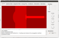
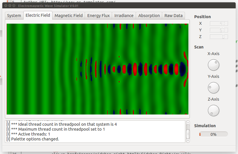
The left figure shows the configuration of a system of size 1,25x5x10 cubic-micrometers using 64x256x512 samples with the VWPM. The run is performed multi-threaded unidirectional with eight threads. The Electric Field is recorder while Magnetic Field as well as Irradiance, the Poynting Vector and the Electromagnetic Flux can be recorded as well by configuration.

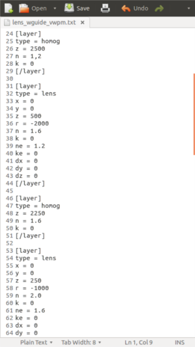
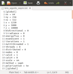
The right figure shows the configuration of various system layers. First a homogeneous layer of 2,5 micrometer thickness and with n=1,2+i0. Second a lens with a radius of -2 micrometer, i.e. a convex lens and then another homogeneous layer followed by another lens. Similar system configurations are usable to simulate and analyse optical lens systems or systems of lenses and mirrors as they might occur in photography or headlights.

[1] M. Fertig and K.-H. Brenner, "Vector wave propagation method", Vol. 27, No. 4/April 2010/J. Opt. Soc. Am., 2010.
[2] M. Fertig, "Vector Wave Propagation Method : Ein Beitrag zum elektromagnetischen Optikrechnen",
Dissertation, Fakultät für Wirtschaftsinformatik und Wirtschaftsmathematik, Universität Mannheim, 2011.
[3] M. Fertig, "The Vector Wave Propagation Method : Ein Beitrag zum elektromagnetischen Optikrechnen",
Vortrag zur Dissertation, Fakultät für Wirtschaftsinformatik und Wirtschaftsmathematik, Universität Mannheim, 18.03.2011.